
This posts introduce basic concepts and derivation of generative modeling.
Generative Models
Depending on whether annotation is available, machine learning mathods can be cetergorized as supervised and unsupervised learning. The different modeling over the distribution $x$ can roughly divide these methods into two catergory: generative and discriminative. In supervised learning, the most common one is discriminative which models the conditional probability $p_\theta(y\mid x)$ parameterized by $\theta$. With $\theta$ learnt from back propagation over the samples, models directly predict $y = p_\theta(y\mid x)$. Gernerative model, on the other hand, models the joint probability of $p(x, y)$ and predict $y=p(y\mid x)=\frac{p(x, y)}{p(x)}$. Knowing what generative model cares about, we focus on the unsupervised generative model that’s used to generate images as real as possible.
Modeling over p(x)
Given a distribution $p_\theta(x)$ parameterized by $\theta$, we denote the true distribution as $p_{\theta^}(x)$. To generate sample $x$ without no annotation as close as possible to $p_{\theta^}(x)$, we want to find the optimal $\theta^$. That is, We want to find a $\theta$ that maximize the log probability of $p_\theta(x)$ with $x\sim p_{\theta^}(x)$.
\[\begin{equation} \theta^* = \operatorname*{argmax}_\theta p_{x\sim p_{\theta^*}(x), \theta}(x) \end{equation}\]Empirically, this equals to maximize the likelihood of joint probability of all training samples:
\[\begin{equation} \theta^* = \operatorname*{argmax}_\theta \prod_{i=1}^{m} p_{\theta}(x_i)\end{equation}\]This can be rewrite as maximization of log likelihood and be approximated by the samples drawn from $p(x)$:
\[\begin{align} \theta^* = \operatorname*{argmax}_\theta \log (p_{x\sim p_{\theta^*}(x), \theta}(x))\\ =\operatorname*{argmax}_\theta \log (\prod_{i=1}^m p_\theta(x_i))\\ =\operatorname*{argmax}_\theta \sum_{i=1}^m \log p_\theta(x_i) \\ \end{align}\]This can also be seem as maximizing the expection of log likelihood with respect to $p_{\theta^\ast}(x)$, which can be rewrite as minimization of cross entropy between the two distributions. This equals to minimization of KL Divergence between the two distributions since the entropy of $p_{\theta^*}(x)$ is fixed as a constant: \(\begin{align} \theta^* &= \operatorname*{argmax}_\theta E_{x\sim p_{\theta^*}(x)}[\log p_\theta (x)]\\ &= \operatorname*{argmin}_\theta \int_x p_{\theta^*}(x) \log \frac{1}{p_\theta (x)} dx\\ \Longleftrightarrow & \operatorname*{argmin}_\theta \int_x p_{\theta^*}(x) \log \frac{1}{p_\theta (x)} dx - \int_x p_{\theta^*}(x) \frac{1}{\log p_{\theta^*}(x)} dx\\ &= \operatorname*{argmin}_\theta \int_x p_{\theta^*}(x) \log \frac{p_{\theta^*}(x)}{p_\theta (x)} dx\\ &= \operatorname*{argmin}_\theta D_{KL}(p_{\theta^*}(x)\mid \mid p_\theta (x)) \end{align}\)
A taxonomy of deep generative models
We refer to NIPS2016 2016 Tutorial on GAN by Ian for taxonomy of generative models.
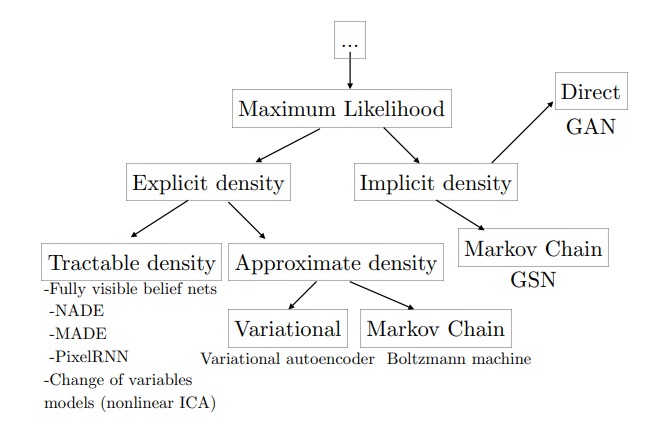
Now that we have the goal: maximization the log likelihood of $p_{x\sim p_{\theta^*}(x), \theta}(x)$. One of the biggest problem is how to define $p_\theta(x)$. Explicit density models define an explicit density function $p_\theta(x)$, which can be directly optimized through backprop. The main difficulty present in explicit density models is designing a model that can capture all of the complexity of the data to be generated while still maintaining computational tractability.